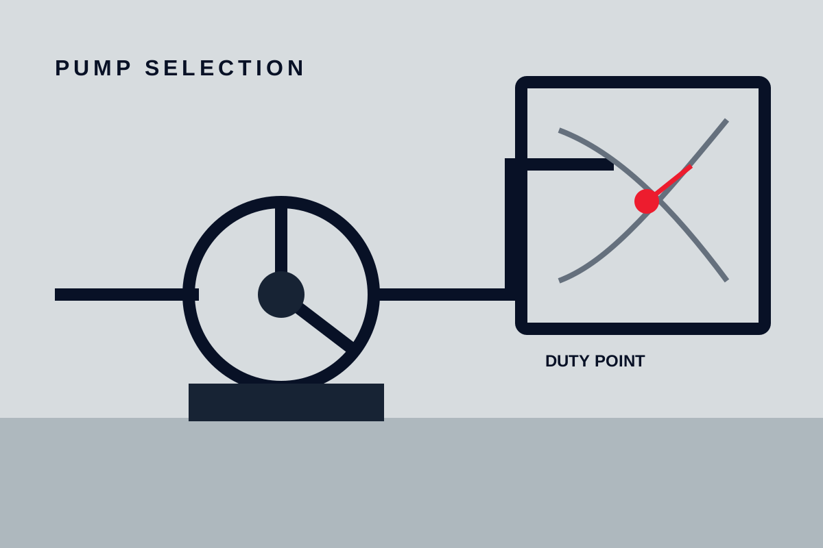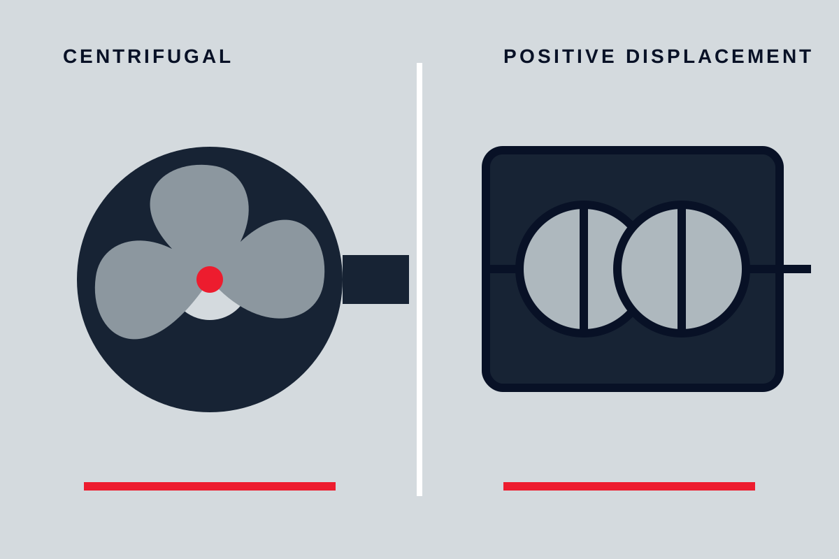


A centrifugal pump’s expected duty point is where its head-versus-flow curve intersects the system curve for a defined operating case. It is not automatically the flow and head listed on a schedule. Before selecting or troubleshooting a pump, you must account for changing liquid levels, pressure boundaries, friction losses, valve positions, pump speed, liquid properties and the manufacturer’s operating limits.
Define the operating cases before drawing the curve
A single nominal flow and head pair rarely describes the full duty. Build separate operating cases for the credible minimum, normal and maximum conditions. Depending on the process, additional cases may be required for startup, filter fouling, emergency operation, parallel-pump operation or unusual tank levels.
Collect these inputs before calculating the system curve:
- Source and destination pressures, including whether vessels are open or pressurized
- Minimum, normal and maximum liquid levels at both system boundaries
- Pipe internal diameters, lengths, elevations, materials and expected roughness
- Fittings, valves, strainers and their operating positions
- Pressure losses through filters, heat exchangers, meters and other equipment
- Required process flow and permitted flow variation
- Liquid density, viscosity, vapor pressure and operating temperature
- Expected pump speed and any proposed speed-control range
- Branch configurations and the number of pumps operating
- Credible changes caused by fouling, wear, maintenance or process reconfiguration
Use the process datasheet, piping and instrumentation diagrams, line list, elevation drawings and control narrative together. A pressure-loss value for a heat exchanger or control valve is useful only when its flow, liquid properties and configuration match the operating case being calculated.
Do not treat the total vertical travel of the pipe as static head. Static head depends on the elevation and pressure difference between the selected system boundaries. A pipe may rise and fall several times without creating an equivalent net static requirement. Pressurized vessels, siphon behavior and changing liquid levels require particularly careful boundary definition.
The manufacturer-produced Wilo system-curve training document provides visual examples of static and friction head. Use such training material to understand the mechanism, but use project data and an approved hydraulic calculation for selection.
Build the pump system curve from static head and losses
The required system head can be represented as:
[ H_{system}(Q) = H_{static} + H_{loss}(Q) ]
Here, (H_{static}) includes the net elevation and pressure-head difference between the system boundaries. (H_{loss}) includes pipe friction and losses through fittings, valves and equipment at flow (Q).
For a transfer between open tanks, the static term is usually related to the difference between the liquid surface elevations. For transfer between pressurized vessels, the pressure difference must also be converted to head using the liquid density. Consequently, the same pressure difference represents a different head for liquids with different densities.
An ideal closed circulation loop generally has no net static elevation head because the rising and falling liquid columns balance. The pump must still overcome flow-dependent resistance. This is why a closed-loop system curve commonly starts near zero head at zero flow, although pressure-control devices or other imposed boundary conditions can change that result.
Darcy-Weisbach is a common method for calculating pipe friction:
[ h_f = f\frac{L}{D}\frac{v^2}{2g} ]
The friction factor (f) depends on Reynolds number and relative roughness. Local losses may be represented with loss coefficients or equivalent lengths, provided the selected method is appropriate and applied consistently.
For turbulent flow in a fixed piping configuration, total resistance is often approximated as proportional to flow squared:
[ H_{system}(Q) \approx H_{static} + KQ^2 ]
This is an approximation, not a universal law. It can become inaccurate when the flow regime changes, viscosity is significant, valves move, branches open or close, or component pressure losses do not follow the same relationship. Manufacturer loss data for filters, valves and heat exchangers may need to be incorporated point by point rather than reduced to one fixed coefficient.
Draw more than one system curve when static conditions or resistance can change. Typical envelopes include:
- Minimum static head with clean equipment and open valves
- Normal levels and normal equipment condition
- Maximum static head with the most restrictive credible valve state
- Fouled-filter or fouled-heat-exchanger operation
- Alternative branch or parallel-pump configurations
Commercial calculation guides, such as the John Brooks system-curve overview, can help illustrate how resistance terms are combined. Any worked values should be recalculated against the project’s own geometry, fluid properties and design method.
Find the intersection with the exact pump curve
Overlay each system curve on the head-versus-flow curve for the exact pump being considered. Confirm the pump model, impeller diameter, rotational speed, test liquid, electrical frequency and curve revision. A curve for another impeller, speed or model is not interchangeable.
The intersection is the predicted steady operating point because it is where the head produced by the pump equals the head required by the system. If the pump produces more head than the system requires at a given flow, flow tends to increase. As system resistance rises with flow and pump head typically declines, the two curves meet.
Consider a purely hypothetical example, not a test result:
[ H_{pump} = 50 - 0.002Q^2 ]
[ H_{system} = 14 + 0.001Q^2 ]
If head is in metres and flow is in cubic metres per hour, equating the two expressions gives a predicted duty of approximately 110 m³/h at 26 m head. This point is valid only for the invented equations. A real selection must use the submitted manufacturer curve and documented system calculations.
The installed point can differ from the prediction if any assumption is wrong. Common causes include incorrect pipe diameter, unexpected valve position, inaccurate equipment-loss data, pump speed error, impeller trimming, wear, air or gas entrainment, changed liquid viscosity, blocked strainers and unrecorded piping modifications.
Check the full operating range, not only one point
A curve intersection establishes a predicted hydraulic balance, but it does not establish that the pump is suitable. Check every credible intersection against the manufacturer’s documentation for the offered configuration.
The review should include:
- Best efficiency point, or BEP
- Preferred and allowable operating ranges
- Hydraulic efficiency at each expected point
- Absorbed power across the operating range
- Motor and drive rating under the specified liquid density
- Net positive suction head required, or NPSHR
- Minimum continuous flow or thermal limits
- Maximum permitted flow and curve-end restrictions
- Speed, impeller and temperature limits
- Restrictions associated with solids, viscosity or gas content
Proximity to BEP is useful, but it does not guarantee acceptable reliability. The manufacturer’s preferred and allowable ranges, together with application-specific mechanical and hydraulic limits, should govern the selection.
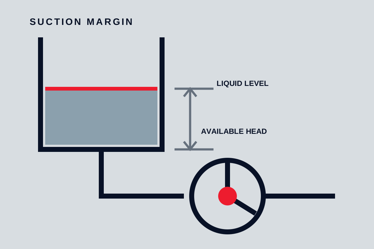
Compare NPSHR with calculated net positive suction head available, or NPSHA, at the most adverse credible suction condition. The NPSHA calculation should account for suction-vessel pressure, liquid level, suction losses and vapor pressure at operating temperature. NPSHR is based on a stated test criterion and is not a complete boundary between cavitating and non-cavitating operation. The required margin must be agreed for the application rather than taken from a universal rule.
Also inspect the power curve over the entire allowed range. A motor selected only for the nominal duty point may be overloaded if the pump moves farther right on its curve under a lower-resistance condition.
Compare how control methods move the duty point
Control arrangements change the operating point in different ways. They should therefore be evaluated on the same pump-and-system diagram.
| Control method | What changes | Main checks |
|---|---|---|
| Throttling valve | Adds resistance and steepens or shifts the system curve | Valve authority, noise, cavitation risk, minimum flow and control range |
| Variable-speed drive | Changes the pump curve by changing rotational speed | Static head, approved speed range, motor cooling, drive limits and control stability |
| Bypass control | Returns some pump discharge flow while process delivery decreases | Pump throughput, recirculation heating, minimum flow and wasted pressure |
| On-off control | Changes run time rather than the running intersection | Starts per hour, tank capacity, pressure cycling and process tolerance |
Throttling can be a practical and stable control method even though it dissipates pressure across the valve. Persistent heavy throttling may indicate excess available head, but it is not proof of pump oversizing without checking the intended control function and actual system curve.
Variable speed shifts the pump head-versus-flow curve. Affinity laws can support preliminary estimates for the same pump under suitable conditions, but they should not be treated as guaranteed performance or energy savings. Static head prevents the operating point from scaling directly with speed, while pump efficiency, motor efficiency and drive losses can also change.
Use manufacturer-approved curves at the proposed speeds where available. Confirm minimum speed, motor cooling, resonance restrictions, minimum continuous pump flow and the drive’s torque and current limits. The Estabrook overview of pump, system and variable-speed curves offers useful commercial background, but model-specific data remain necessary.
Bypass control protects minimum pump flow or supports a process requirement, but recirculating liquid does not necessarily reduce pump throughput. On-off control changes how long the pump runs; while running at fixed speed and valve position, the pump still settles near the intersection of its pump curve and the active system curve.
Recognize oversizing from operation, not the nameplate
A pump is not proven oversized merely because its motor has a high nameplate rating or its published maximum flow exceeds process demand. Oversizing is better diagnosed from the resulting operating range and control burden.
Indicators worth investigating include:
- A control valve remaining heavily throttled during representative operation
- Sustained operation outside the manufacturer’s preferred range
- Large bypass flow during normal demand
- Unstable flow or pressure control
- Measured delivery consistently exceeding process requirements
- An impeller diameter or speed substantially above that required by the verified system curve
Each sign has alternative explanations. A throttled valve may be performing its intended pressure-control function. A high measured flow may indicate lower system resistance rather than an oversized original selection. Low flow can result from fouling, blockage, incorrect rotation, wear or higher-than-expected static head.
Review trends for flow, pump speed, suction and discharge pressure, valve position, tank levels and motor input across representative operating states. Compare these records with commissioning data, maintenance history and any piping or impeller changes. Instrument calibration and valve configuration should be verified before revising the pump selection.
Verify the installed duty point safely
Field measurements can test the assumptions, but suction and discharge pressure readings alone do not automatically establish pump head. For incompressible liquid, pump head can be estimated from:
[ H = \frac{p_d-p_s}{\rho g} + \frac{v_d^2-v_s^2}{2g} + (z_d-z_s) ]
The calculation requires pressure-tap elevations, pipe velocities, actual liquid density and stable operating conditions. Record instrument ranges, calibration status and measurement uncertainty. Pressure taps close to the pump nozzles are generally preferable where the pump manufacturer’s method and installation permit them.
A practical verification sequence is:
- Confirm the installed pump model, impeller diameter, rotation and actual speed.
- Verify valve states, branch configuration and process conditions.
- Record stable suction pressure, discharge pressure, flow, speed, liquid temperature and density.
- Correct the pressure difference for elevation and velocity effects where material.
- Plot the resulting point against the applicable pump curve.
- Compare it with the calculated system curve and investigate discrepancies.
- Repeat at enough operating states to evaluate the expected range, rather than relying on one reading.
Before opening guards, accessing couplings, removing instruments or performing intrusive inspection, isolate electrical and mechanical energy, depressurize and drain the relevant system, and follow the manufacturer’s instructions and site safety procedures.
Set acceptance criteria before ordering
Require quotations to identify the guaranteed duty, exact pump model, curve revision, impeller diameter, speed and test liquid. The submission should also show the operating-range boundaries, absorbed power, efficiency, NPSHR and applicable minimum-flow restrictions.
State the required test basis and acceptance tolerances in the purchase specification and inspection plan before manufacture or testing. Do not assume that a generic catalogue curve is a guaranteed curve for the offered configuration.
The final selection rule is bounded: accept the pump only when all credible system-curve intersections fall within the manufacturer’s permitted range, the driver covers maximum absorbed power, the suction assessment provides the agreed NPSH margin, and the supplier documents the exact offered configuration and performance basis. If those conditions cannot be demonstrated, revise the pump, impeller, speed, controls or system assumptions before purchase.
Frequently asked questions
Why does a centrifugal pump not automatically operate at its rated flow?
The running flow is established by the intersection of the active pump and system curves. A scheduled or rated flow is a specified selection point, not a flow that the pump independently enforces. Changed resistance, static head or speed moves the intersection.
Does a closed-loop piping system have static head?
An ideal closed circulation loop generally has no net static elevation head because the liquid columns balance. The pump still overcomes friction and equipment losses. Pressure-control boundaries, open sections or an incorrectly defined system boundary can introduce an additional static term.
How does a variable-frequency drive move the duty point?
Changing speed changes the pump curve, and the new curve intersects the existing system curve at a different point. The movement depends on the amount of static head, the system’s resistance relationship and changes in pump efficiency. It should be checked with approved speed-specific data where possible.
Can suction and discharge pressure readings confirm the actual duty point?
They can support the calculation of pump head when tap locations, elevation difference, velocity effects, liquid density, calibration and operating stability are known. A flow measurement and actual speed are also needed to place the field point meaningfully on the pump curve.